Lana Del Ray: Song Discography

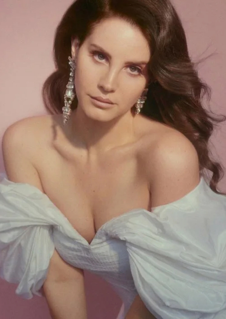
Лана Дель Рей — американская певица, автор песен и модель. Она начала свою карьеру в конце 2000-х, взорвав чарты с дебютным альбомом Born to Die в 2012 году, где смешала гламурный поп с элементами трип-хопа, дрим-попа и блюза. Её музыкальный стиль уникален: меланхоличные, кинематографичные мелодии с лирикой о любви, ностальгии, голливудских мечтах и тёмной романтике, часто с отсылками к американской культуре 1950–60-х, барокко-попом и альтернативным R&B. В 2024 году, спустя более 12 лет карьеры, она укрепила статус иконы, выпустив альбом Did You Know That There’s a Tunnel Under Ocean Blvd, который получил восторженные отзывы и новые хиты. Она также успешно провела несколько мировых туров, собирая стадионы. В связи с многолетней популярностью певицы, я решила провести анализ её дискографии: прослушивания треков, годы выпуска и альбомы с наибольшим количеством хитов в датасете.

Цвета отсылают к обложке одного из самых популярных альбомов певицы — BORN TO DIE

import pandas as pd import matplotlib.pyplot as plt import difflib fn = "ldr_discography_released.csv" df = pd.read_csv(fn, encoding='utf-8', dtype=str) candidates = ['album', 'album_title', 'album name', 'album_name', 'Album', 'Album Title', 'Album_Name', 'release', 'album_title'] def normalize(name): return name.lower().replace(' ', '').replace('_', '').replace('-', '') cols = df.columns.tolist() for cand in candidates: if cand in cols: album_col = cand break else: norm_map = {normalize(c): c for c in cols} found = None for cand in candidates: nc = normalize(cand) if nc in norm_map: found = norm_map[nc] break if found: album_col = found else: names = cols close = difflib.get_close_matches("album", names, n=1, cutoff=0.6) close2 = difflib.get_close_matches("albumtitle", names, n=1, cutoff=0.6) if close: album_col = close[0] elif close2: album_col = close2[0] else: raise ValueError(f"Не найдена колонка с альбомами. Доступные колонки: {cols}\n" "Если в вашем файле колонка называется по-другому — укажите её явно в переменной album_col.") print(f"Использую колонку: {album_col}") counts = df[album_col].dropna().astype(str).str.strip().replace('', '').value_counts() total = counts.sum() counts = counts.sort_values(ascending=False) print("Треков по альбомам:") print(counts) plt.rcParams['font.family'] = 'DejaVu Sans' threshold_pct = 1.0
small = counts[counts / total * 100 < threshold_pct] if len(small) > 0: other = small.sum() counts = counts[counts / total * 100 >= threshold_pct] counts['Other'] = other pie_colors = ['

759CD9', '

import plotly.graph_objects as go import plotly.io as pio top_n = 20 colors = ['

759CD9', '

fig = go.Figure(go.Bar( x=df_plot['song_page_views'], y=df_plot['label'], orientation='h', marker=dict(color=color_cycle), hovertemplate='%{y}
Просмотры: %{x}' )) fig.update_layout( title=f'Top {top_n} треков по числу просмотров', xaxis_title='Просмотры (song_page_views)', yaxis_title='', margin=dict(l=300, r=40, t=60, b=40), height=40*top_n + 200 ) out_file = 'top_tracks_histogram.html' fig.write_html(out_file, include_plotlyjs='cdn') print('Топ-10 треков по просмотрам:') print(df_sorted[['song_title', 'artists_str', 'song_page_views']].head(10).to_string(index=False)) print(f"\nИнтерактивный график сохранён в файл: {out_file}") fig, out_file

import plotly.express as px import pandas as pd top_n = 30
colors = ['

759CD9', '

selected = df.sort_values('song_page_views', ascending=False).head(top_n).copy() selected = selected.reset_index(drop=True) selected['color_group'] = selected.index % len(colors) color_map = {i: colors[i] for i in range(len(colors))} selected['color_hex'] = selected['color_group'].map(color_map) print(f"Selected top {top_n} tracks by song_page_views:\n") print(selected[['song_title','song_artists','song_release_date','song_page_views','color_hex']])

fig = px.scatter( selected, x='song_release_date', y='song_page_views', color='color_group', color_discrete_map={str(k): v for k, v in color_map.items()}, hover_data=['song_title','song_artists','song_release_date','song_page_views'], title=f'Релизы {top_n} самых популярных треков (по просмотрам)', labels={'song_release_date': 'Дата релиза', 'song_page_views': 'Просмотры'}, height=600 ) size_ref = selected['song_page_views'].max() / 40 fig.update_traces(marker=dict(size=[max(6, v/size_ref) for v in selected['song_page_views']], line=dict(width=1, color='DarkSlateGrey')))

fig.update_layout(showlegend=True) fig.write_html(output_html, include_plotlyjs='cdn') print(f"\nСохранён файл с интерактивной диаграммой: {output_html}") fig

import plotly.express as px import pandas as pd

N = 10
colors = ['

759CD9', '

top_n = df.sort_values('song_page_views', ascending=False).head(N).copy() top_n['album_title'] = top_n['album_title'].fillna('Unknown Album')

counts = top_n['album_title'].value_counts().reset_index() counts.columns = ['album_title', 'count'] print('Распределение топ-{} треков по альбомам:'.format(N)) print(counts.to_string(index=False)) fig = px.pie(counts, names='album_title', values='count', title=f'Распределение топ-{N} треков по альбомам', color_discrete_sequence=colors) fig.update_traces(textposition='inside', textinfo='percent+label')

out_path = 'top_tracks_albums_pie.html' fig.write_html(out_path, include_plotlyjs='cdn') print(f"График сохранён в файл: {out_path}") fig

Я нашла и провела анализ датасета, в котором содержится информация о дискографии популярной исполнительницы Ланы Дель Рей.

В результате работы я создала четыре диаграммы, акцентирующие внимание на самых важных пунктах: популярных песнях и альбомах, датах релизов треков и т.д.